
Monte Carlo simulation acts as the cornerstone for robust financial modeling in the [currentmonth] [currentyear] currency market environment. By generating thousands of hypothetical equity curves based on historical trade outcomes, professional traders distinguish between a strategy with genuine statistical edge and one that merely benefited from recent market luck. This method moves beyond standard backtesting by accounting for the inherent randomness in the order of trade sequences, ensuring that your risk management parameters survive even the most hostile sequences of consecutive losses. Relying solely on historical profit factors often blinds investors to potential ruin. Implementing rigorous simulation protocols allows for the precise calculation of ruin probability, helping you adjust your position sizing to maintain portfolio longevity despite inevitable market volatility and adverse trade clusters.
Successful trading is rarely about predicting the next tick but rather about managing the distribution of outcomes over a series of future transactions. This analytical framework provides the mathematical certainty required to scale a strategy with confidence. When you simulate the variance of your trade distribution, you effectively stress test your account equity against the worst-case scenarios allowed by your current risk model.
- Explore tracking trade logs using our free Excel trading journal template.
- Explore calculating exact dollar margin requirements using the multi-asset margin calculator.
- Explore evaluating N-unit position sizing in the Turtle trading system rules.
Understanding the Mechanics of Monte Carlo Simulation
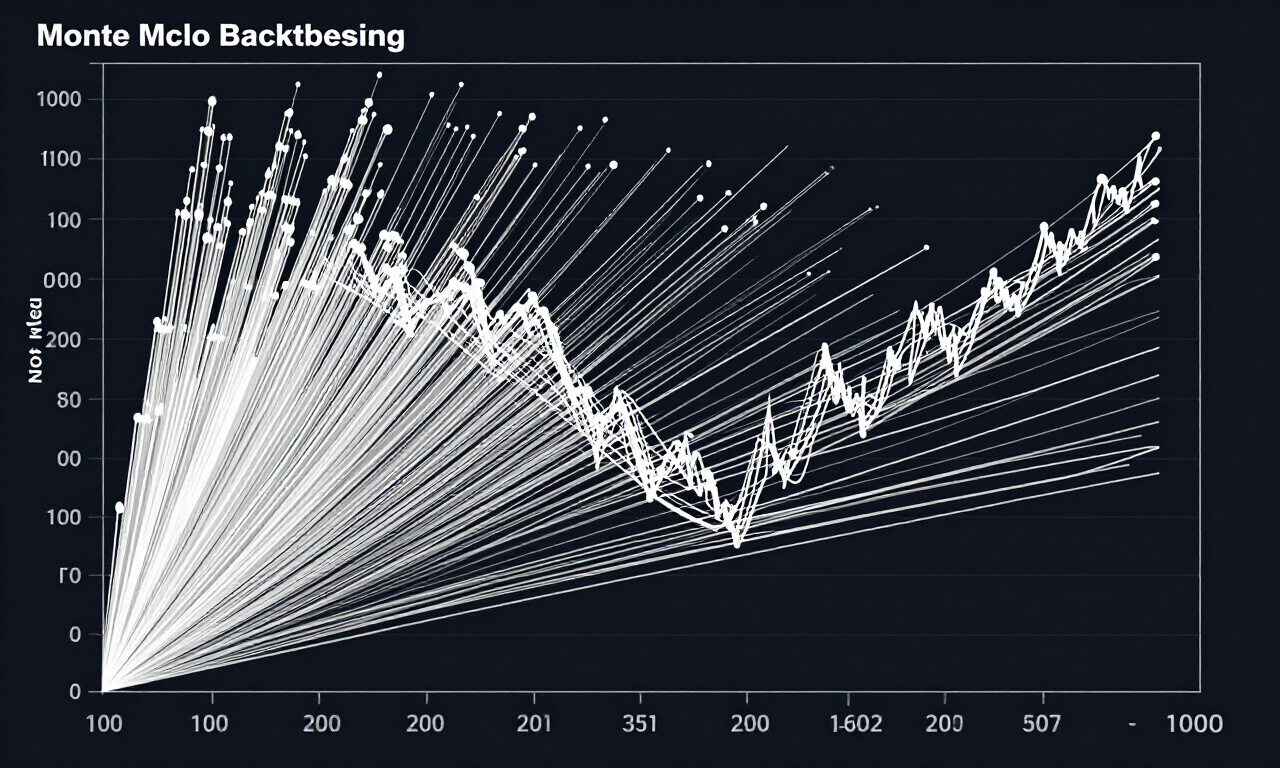
Monte Carlo simulation is a computational algorithm that repeatedly generates synthetic equity paths by randomly shuffling your historical trade results. This process creates thousands of unique equity curves, allowing traders to observe the potential range of drawdowns and profitability rather than relying on a single, fixed, and potentially deceptive historical backtest outcome.
Most traders evaluate their performance using a linear approach. They look at a backtest report, see a profit factor of 2.0, and assume the strategy is solid. However, the sequence of wins and losses is rarely fixed. If you move your three largest losing trades to the beginning of your sequence, does your account hit a margin call?
Statistical probability dictates that clusters of losses are inevitable. Even a strategy with a 70% win rate will occasionally experience a string of consecutive losses. The simulation process isolates these clusters to reveal if your drawdown tolerance matches your actual capital capacity. By calculating the variance in your trade win/loss distribution, you gain insight into the “true” risk of the account.
Practitioner Pro-Tip: Never run a simulation on fewer than 100 historical trades. A sample size smaller than 100 will produce results heavily influenced by noise rather than the statistical edge of your system.
Modern platforms like MetaTrader 5 or custom Python scripts allow for this depth of analysis. When you feed your trade list into the simulation engine, you essentially treat your past performance as a probability distribution. The algorithm draws from this distribution to build new realities. If 5% of your simulated equity curves result in account ruin, you know that your position sizing is mathematically aggressive regardless of your past success.
Equity Curve Drawdown Analysis
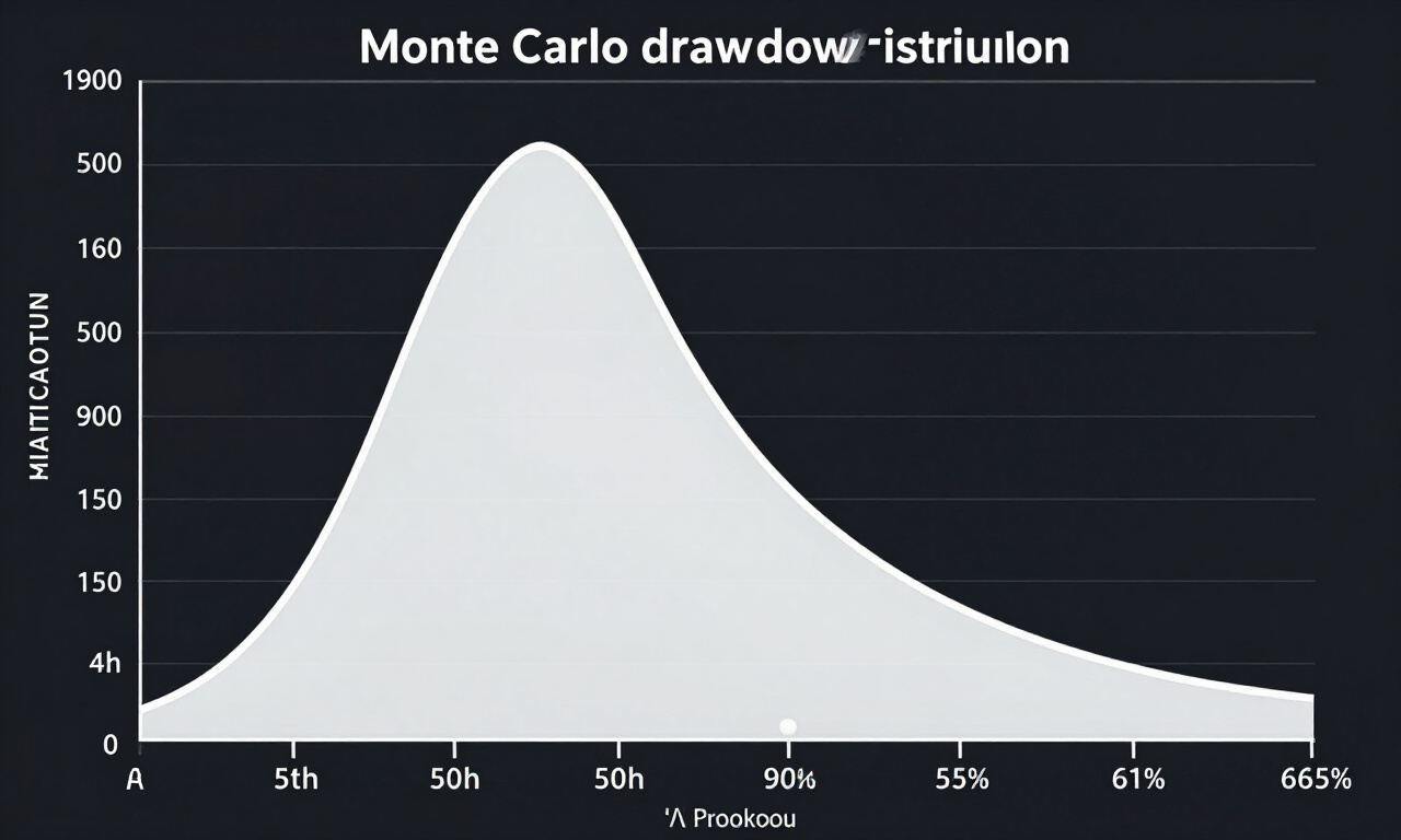
Equity curve drawdown analysis measures the peak-to-trough decline of your account balance during simulated trading sessions. By evaluating the depth and duration of these declines across thousands of iterations, you determine the maximum probable drawdown your account might face, ensuring your capital allocation remains safe during adverse streaks.
Drawdown is the silent killer of trading careers. Many participants focus exclusively on the equity slope, ignoring the jagged path taken to reach a target. A system that makes 50% returns but faces a 40% drawdown is often discarded by professional capital allocators because the psychological and financial toll is too extreme.
When you use Monte Carlo simulations to analyze your equity curve, you are looking for the ‘Worst Case’ scenarios. If your backtest shows a 10% maximum drawdown, but your simulation reveals that 10% of your tests show a 30% drawdown, you must plan for that 30% event. This knowledge changes how you allocate capital to your forex trading account.
- Calculate the ‘Maximum Drawdown’ across all iterations.
- Identify the frequency of ‘Drawdown Durations’ (how long the account stays below peak).
- Compare the median drawdown against the worst-case 95th percentile outcome.
- Adjust position size coefficients to keep the 95th percentile drawdown within your risk threshold.
By mapping out these probabilities, you move from speculative betting to institutional risk management. You no longer hope for a streak of winners; you prepare for the statistical necessity of a streak of losers. This structural shift is what separates hobbyists from consistent professional traders who manage institutional portfolios.
Simulating Trade Sequences
Simulating trade sequences involves randomizing the temporal order of your recorded trade outcomes to test the impact of variance. By ignoring the original chronological order, you isolate the probability of experiencing a cluster of negative results, which often causes account failure even in profitable, long-term trading systems.
If your strategy produced a win-loss-win-loss sequence in history, a Monte Carlo simulation will test the same system with a loss-loss-loss-win sequence. This is critical because humans suffer from cognitive biases that make us overestimate our ability to handle losses. If you start your account with three consecutive full-position losses, your psychology may force you to abandon a perfectly good system.
This test reveals the ‘breaking point’ of your account. If you see that your system has a 2% probability of hitting a 50% drawdown, you must decide if that 2% risk is acceptable. In professional circles, this is often the moment a trader decides to decrease their risk per trade to 0.5% or 1%, effectively ‘smoothing’ the curve and reducing the impact of variance.
Quantifying Probability of Ruin
The probability of ruin is a mathematical calculation determining the likelihood that an account will reach zero or a specified minimum threshold. Through Monte Carlo iteration, you assign a percentage value to the risk of catastrophic loss, allowing for the scientific adjustment of risk parameters before live execution.
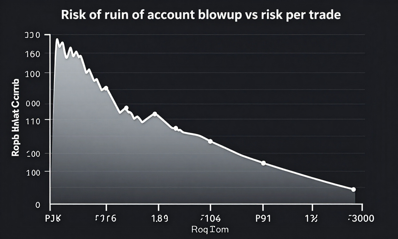
Most traders find that their subjective view of risk is vastly different from the objective reality. You might believe that risking 5% per trade is ‘aggressive but manageable.’ A Monte Carlo simulation might show that your probability of ruin is 15% over the next 500 trades. This discrepancy is where many traders fail to achieve longevity.
To calculate this, you need your ‘Win Rate’, ‘Average Win Size’, ‘Average Loss Size’, and ‘Total Number of Trades’. The simulation will run 5,000 versions of your next 500 trades. You count how many of those 5,000 versions resulted in the account dropping below your ruin threshold. That percentage is your probability of ruin.
If the result is higher than 1%, it is time to optimize. Optimization here does not mean finding a ‘better’ indicator. It means lowering your trade exposure. By halving your position size, your probability of ruin often drops exponentially rather than linearly, providing a massive buffer for account safety.
Refining Position Sizing Models
Refining position sizing through simulation involves adjusting the percentage of capital committed to each trade based on the distribution of previous outcomes. By observing how different sizing coefficients affect the equity curve variability, you can mathematically determine the optimal size that maximizes growth while keeping drawdowns within acceptable limits.
Optimal F is a classic concept in position sizing that seeks to maximize the geometric growth of an account. However, Optimal F is notoriously volatile and frequently leads to severe drawdowns. Using Monte Carlo simulation, you can find a ‘fractional’ Optimal F, which offers a safer path to growth while respecting your personal risk tolerance.
When you run your simulations, keep track of your ‘Growth Rate’ for different risk percentages. You will notice that as you increase your risk, your expected growth increases to a point, after which it drops off as the frequency of massive drawdowns wipes out previous gains. This is the ‘peak of the curve’ you want to stay near without crossing the line into excessive risk.
Always incorporate slippage and spread widening into your simulations. Many backtests are overly optimistic because they assume perfect execution at the exact price point. When you add a margin of error for execution, your simulation becomes a real-world tool that predicts actual performance rather than theoretical perfection.
Integrating Simulation into Trading Workflows
Integration involves moving simulation from an occasional check to a mandatory step in your strategy deployment pipeline. Every time a system produces a new set of trade data, you must run it through the simulator to verify that the risk profile remains within your institutional mandate for account safety.
Trading as a business requires consistent feedback loops. You should not consider a system ‘tradeable’ until it has passed the Monte Carlo litmus test. This includes testing against various market regimes, such as high-volatility environments and low-volatility periods, to see if the trade sequence outcomes are robust enough to withstand regime shifts.
Make sure to utilize historical data from the current year to ensure your parameters are not based on outdated market dynamics. Currency pairs have distinct personalities; the volatility of the GBPJPY is vastly different from the EURUSD. Your simulation must reflect the specific asset class you intend to trade.
Document every simulation result. Keeping a log of your risk metrics—like expected drawdown vs. realized drawdown—will help you refine your models over time. If you notice a consistent deviation between your simulations and live performance, it likely indicates that your transaction costs or slippage assumptions need to be adjusted upward.
Frequently Asked Questions
Frequently asked questions regarding Monte Carlo simulation cover the practical application of risk modeling and equity curve analysis. By clarifying the necessity of these statistical tests, traders can move away from intuition-based decision making and adopt a rigorous, evidence-based approach to managing their capital in the competitive forex market.
- How many simulations should I run for a robust result?
A minimum of 1,000 to 5,000 iterations is recommended. This provides enough data to generate a stable probability distribution curve and helps identify the outliers that represent the 95th and 99th percentile of drawdown scenarios. - Does Monte Carlo simulation guarantee future performance?
No. It only provides a statistical probability based on historical data. Markets evolve, and correlations change. It is a risk management tool, not a crystal ball for predicting future profit cycles or market movements. - What is the biggest mistake traders make with simulations?
The most common error is ignoring transaction costs. Many traders simulate raw price movement without accounting for spreads, commissions, and slippage. This leads to an overestimation of the system’s edge and an underestimation of potential drawdown depths. - How often should I re-run these simulations?
Perform a new simulation whenever you have a statistically significant increase in trade history (e.g., every 50-100 trades). Additionally, re-run simulations whenever you significantly adjust your trading strategy or risk management parameters to ensure your updated model is still viable.